
Microsoft Excel is used by millions of people every day. Since it came into existence, Excel has been the dominant spreadsheet tool.
While there are other spreadsheet tools available in the market (such as Open Office, Google Sheets, LibreOffice), nothing comes even close to the features and capabilities that Excel offers.
In this article, I will share five Excel tricks that can help you save a lot of time and make you highly productive.
1. Speedup Data Entry With Drop Down Lists
While Excel is much more than a data entry tool, a lot of people use it to maintain records and data.
If your work involves entering data in Excel, using an Excel drop-down list can speed it up.
A drop-down menu allows you to select from a pre-defined list of items. You just need to select the relevant item from the list and it automatically gets entered in the cell.
Apart from saving time, this also ensures that there are no errors in the data entry (such as spelling mistakes or inconsistent data entry).
Here are the steps to create a drop-down list in Excel:
- Create a list of the items that you want in the drop down. For example, if you want to a list of products, create a list in the spreadsheet with the names of the products.
- Select the cell in which you want the drop-down. If you want the drop down in multiple cells, select all these cells.
- Go to the Data tab and select the Data Validation option.

- In the Data Validation dialog box, within the settings tab, select List as the validation criteria.
- Click on the source field, and use the mouse to select the cells that have the items that you want in the drop down.
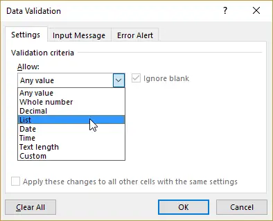
- Click OK.
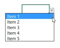
The steps above will create a drop down list in the selected cell(s). You will see a small downward pointing arrow when you select a cell that has the drop down.
Just click on the arrow icon and the drop-down list would appear.
Now you can choose the item from it and it will automatically be entered in the cell.
2. Quickly Remove Duplicates in Excel
If you work with data in Excel, you would know the issues duplicate data points can create.
This is especially the case when you get the data from a colleague/client, or you consolidate it from multiple sources.
Here are the steps you can use to delete all the duplicate records in a few seconds.
- Select the entire data set.
- Go to the Data tab and click on the Remove Duplicates option.

- In the Remove Duplicate dialog box, select the columns from which you want to delete the duplicates. If you want, you can select all the columns by clicking on the ‘Select All’ button.
- Click OK.
As soon as you do this, Excel removes the duplicate records and show you the number of records it has deleted (in a prompt).
Pro Tip: Create a backup of the original dataset as removing duplicates will alter the data set.
3. Use Freeze Panes When Working with Large Datasets
If you have worked with large datasets in Excel, you know the pain of scrolling back and forth.
As soon as you scroll to the right or scroll down, the headers disappear. This makes it difficult to know what a data point refers to (as you can’t see the headers).
Freeze Panes option makes it easy by locking the headers so that these are always visible.
Here are the steps to freeze the headers:
- Select the cell above which you want to freeze the rows and to the left of which you want to freeze the columns. For example, if you want to freeze the top row and the left-most column, select cell B2.
- Go to the View tab and click on the Freeze Panes option.

Now whenever you go to the scroll to the right or scroll down, the headers would always be visible.
[Read also: How Excel Can Boost Your Productivity at Work]
4. Quickly Highlight Blank Cells In Excel
If you create data models or perform calculations in Excel, it’s a good practice to make sure there are no blank cells in your data set.
Blank cells may lead to errors or unexpected results.
Here are the steps to quickly highlight blank cells in a dataset:
- Select the dataset in which you want to highlight the blank cells.
- Press the F5 key from your keyboard. This will open the ‘Go To’ dialog
- Click on the Special button

- In the ‘Go To Special’ dialog box, select Blanks.

- Click OK.
The above steps would select all the blank cells in the data set.
Now you can highlight these by giving it a color.
5. Quickly Insert Comments in Cells Using a Keyboard Shortcut
If you review other people’s work or need to add some commentary to data points/cells, inserting a comment is the way to go.
You can quickly insert the comment in a cell using the keyboard shortcut Shift + F2.
This would insert the comment and place the cursor in the comment so you can enter the text in it.
Once you are done entering the comment, press the Escape key or click anywhere in the worksheet.
You can also use the same keyboard shortcut to edit comments in a cell.
